Range partitioning

A natural way to partition the metrics table is to range partition on the time column. Let’s assume that we want to have a partition per year, and the table will hold data for 2014, 2015, and 2016. There are at least two ways that the table could be partitioned: with unbounded range partitions, or with bounded range partitions.

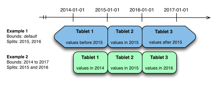
The image above shows the two ways the metrics table can be range partitioned on the time column. In the first example (in blue), the default range partition bounds are used, with splits at 2015-01-01 and 2016-01-01. This results in three tablets: the first containing values before 2015, the second containing values in the year 2015, and the third containing values after 2016. The second example (in green) uses a range partition bound of [(2014-01-01), (2017-01-01)], and splits at 2015-01-01 and 2016-01-01. The second example could have equivalently been expressed through range partition bounds of [(2014-01-01), (2015-01-01)], [(2015-01-01), (2016-01-01)], and [(2016-01-01), (2017-01-01)], with no splits. The first example has unbounded lower and upper range partitions, while the second example includes bounds.

Each of the range partition examples above allows time-bounded scans to prune partitions falling outside of the scan’s time bound. This can greatly improve performance when there are many partitions. When writing, both examples suffer from potential hot-spotting issues. Because metrics tend to always be written at the current time, most writes will go into a single range partition.

The second example is more flexible, because it allows range partitions for future years to be added to the table. In the first example, all writes for times after 2016-01-01 will fall into the last partition, so the partition may eventually become too large for a single tablet server to handle.