Tuning Spark Shuffle Operations
A Spark dataset comprises a fixed number of partitions, each of which comprises a number
of records. For the datasets returned by narrow transformations, such as
map and filter, the records required to compute the
records in a single partition reside in a single partition in the parent dataset.
Each object is only dependent on a single object in the parent. Operations such as
coalesce can result in a task processing multiple input partitions, but
the transformation is still considered narrow because the input records used to compute
any single output record can still only reside in a limited subset of the partitions.
Spark also supports transformations with wide
dependencies, such as groupByKey and
reduceByKey. In these dependencies, the data required
to compute the records in a single partition can reside in many
partitions of the parent dataset. To perform these transformations,
all of the tuples with the same key must end up in the same partition,
processed by the same task. To satisfy this requirement, Spark performs a
shuffle, which transfers data around the cluster and results in a
new stage with a new set of partitions.
For example, consider the following code:
sc.textFile("someFile.txt").map(mapFunc).flatMap(flatMapFunc).filter(filterFunc).count()
It runs a single action, count, which depends on a sequence of three
transformations on a dataset derived from a text file. This code runs in a single stage,
because none of the outputs of these three transformations depend on data that comes
from different partitions than their inputs.
In contrast, this Scala code finds how many times each character appears in all the words that appear more than 1,000 times in a text file:
val tokenized = sc.textFile(args(0)).flatMap(_.split(' '))
val wordCounts = tokenized.map((_, 1)).reduceByKey(_ + _)
val filtered = wordCounts.filter(_._2 >= 1000)
val charCounts = filtered.flatMap(_._1.toCharArray).map((_, 1)).reduceByKey(_ + _)
charCounts.collect()
This example has three stages. The two reduceByKey transformations each
trigger stage boundaries, because computing their outputs requires repartitioning the
data by keys.
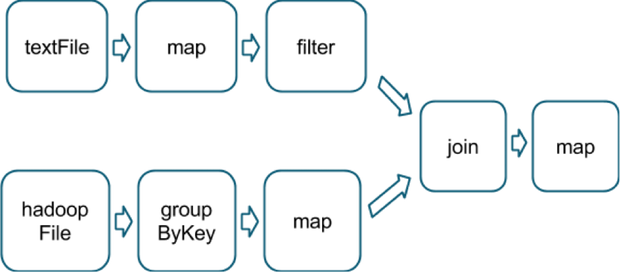
A final example is this more complicated transformation graph, which includes a
join transformation with multiple dependencies:
The pink boxes show the resulting stage graph used to run it:
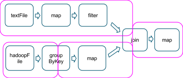
At each stage boundary, data is written to disk by tasks in the parent
stages and then fetched over the network by tasks in the child stage.
Because they incur high disk and network I/O, stage boundaries can be
expensive and should be avoided when possible. The number of data
partitions in a parent stage may be different than the number of
partitions in a child stage. Transformations that can trigger a stage
boundary typically accept a numPartitions argument, which
specifies into how many partitions to split the data in the child stage.
Just as the number of reducers is an important parameter in MapReduce
jobs, the number of partitions at stage boundaries can determine an
application's performance. "Tuning the Number of Partitions" describes how
to tune this number.