Introduction to Production Machine Learning
Machine learning (ML) has become one of the most critical capabilities for modern businesses to grow and stay competitive today. From automating internal processes to optimizing the design, creation, and marketing processes behind virtually every product consumed, ML models have permeated almost every aspect of our work and personal lives.
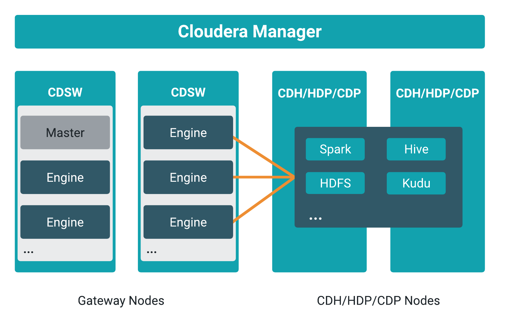
Each CDSW installation enables teams of data scientists to develop, test, train and ultimately deploy machine learning models for building predictive applications all on the data under management within the enterprise data cloud. Each ML workspace supports fully-containerized execution of Python, R, Scala, and Spark workloads through flexible and extensible engines.
Core capabilities
-
Seamless portability across private cloud, public cloud, and hybrid cloud powered by Kubernetes
-
Fully containerized workloads - including Python, and R - for scale-out data engineering and machine learning with seamless distributed dependency management
-
High-performance deep learning with distributed GPU scheduling and training
-
Secure data access across HDFS, cloud object stores, and external databases
CDSW users
-
Data management and data science executives at large enterprises who want to empower teams to develop and deploy machine learning at scale.
-
Data scientist developers (use open source languages like Python, R, Scala) who want fast access to compute and corporate data, the ability to work collaboratively and share, and an agile path to production model deployment.
-
IT architects and administrators who need a scalable platform to enable data scientists in the face of shifting cloud strategies while maintaining security, governance, and compliance. They can easily provision environments and enable resource scaling so they - and the teams they support - can spend less time on infrastructure and more time on innovation.
Challenges with model deployment and serving
After models are trained and ready to deploy in a production environment, lack of consistency with model deployment and serving workflows can present challenges in terms of scaling your model deployments to meet the increasing numbers of ML use-cases across your business.
Many model serving and deployment workflows have repeatable, boilerplate aspects that you can automate using modern DevOps techniques like high-frequency deployment and microservices architectures. This approach can enable machine learning engineers to focus on the model instead of the surrounding code and infrastructure.
Challenges with model monitoring
Machine Learning (ML) models predict the world around them which is constantly changing. The unique and complex nature of model behavior and model lifecycle present challenges after the models are deployed.
You can monitor the performance of the model on two levels: technical performance (latency, throughput, and so on similar to an Application Performance Management), and mathematical performance (is the model predicting correctly, is the model biased, and so on).
There are two types of metrics that are collected from the models:
Time series metrics: Metrics measured in-line with model prediction. It can be useful to track the changes in these values over time. It is the finest granular data for the most recent measurement. To improve performance, older data is aggregated to reduce data records and storage.
-
track_metrics: Tracks the metrics generated by experiments and models.
-
read_metrics: Reads the metrics already tracked for a deployed model, within a given window of time.
-
track_delayed_metrics: Tracks metrics that correspond to individual predictions, but aren’t known at the time the prediction is made. The most common instances are ground truth and metrics derived from ground truth such as error metrics.
-
track_aggregate_metrics: Registers metrics that are not associated with any particular prediction. This function can be used to track metrics accumulated and/or calculated over a longer period of time.
The following two use-cases show how you can use these functions:
-
Tracking accuracy of a model over time
-
Tracking drift
Use case 1: Tracking accuracy of a model over time
Consider the case of a large telco. When a customer service representative takes a call from a customer, a web application presents an estimate of the risk that the customer will churn. The service representative takes this risk into account when evaluating whether to offer promotions.
The web application obtains the risk of churn by calling into
a model hosted on CDSW. For each prediction thus obtained, the web application records the
UUID into a datastore alongside the customer ID. The prediction itself is tracked in CDSW
using the track_metrics function.
At some point in the future, some customers do in fact churn. When a customer churns, they or another customer service representative close their account in a web application. That web application records the churn event, which is ground truth for this example, in a datastore.
An ML engineer who works at the telco wants to continuously
evaluate the suitability of the risk model. To do this, they create a recurring CDSW job.
At each run, the job uses the read_metrics
function to read all the predictions that were tracked in the last interval. It also reads
in recent churn events from the ground truth datastore. It joins the churn events to the
predictions and customer ID’s using the recorded UUID’s, and computes an Receiver operating
characteristic (ROC) metric for the risk model. The ROC is tracked in the metrics store
using the track_aggregate_metrics
function.
The ground truth can be stored in an external datastore, such as Cloudera Data Warehouse or in the metrics store.
Use case 2: Tracking drift
Instead of or in addition to computing ROC, the ML engineer may need to track various types of drift. Drift metrics are especially useful in cases where ground truth is unavailable or is difficult to obtain.
The definition of drift is broad and somewhat nebulous and practical approaches to handling it are evolving, but drift is always about changing distributions. The distribution of the input data seen by the model may change over time and deviate from the distribution in the training dataset, and/or the distribution of the output variable may change, and/or the relationship between input and output may change.
All drift metrics are computed by aggregating batches of
predictions in some way. As in the use case above, batches of predictions can be read into
recurring jobs using the read_metrics
function, and the drift metrics computed by the job can be tracked using the track_aggregate_metrics function.