Networking Considerations for Virtual Private Clusters
Minimum Network Performance Requirements
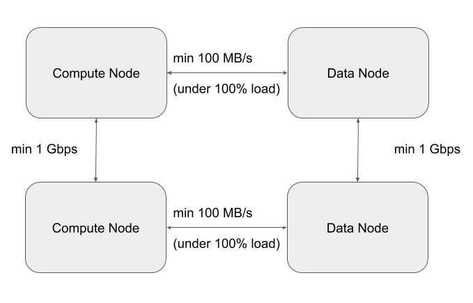
A Virtual Private Cluster deployment has the following requirements for network performance:
- A worst case IO throughput of 100MB/s , i.e., 1 Gbp/s of network throughput (sustained) between any compute node and any storage node. To achieve the worst case, we will measure throughput when all computenodes are reading/writing from the storage nodes at the same time. This type of parallel execution is typical of big data applications.
- A worst case network bandwidth of 1Gbps between any two workload cluster Nodes or any two base cluster Nodes.
The following picture summarizes these requirements:
Sizing and designing the Network Topology
Minimum and Recommended Performance Characteristics
This section can be used to derive network throughput requirements, following the minimum network throughputs outlined in the table below.
| Tier | Minimum Per-Node Storage IO throughput (MB/s) | Minimum per-Node network throughput (Gbps) (EW + NS) | Recommended per-Node Storage IO throughput (MB/s) | Recommended per-Node network throughput (Gbps) (EW + NS) |
| Compute (This can be virtualized or bare-metal) | 100 | 2 | 200 | 4 |
| Storage (This can be virtualized or bare-metal) | 400 | 8 | 800 | 16 |
Network Topology Considerations
The preferred network topology is spine-leaf with as close to 1:1 over subscription between leaf and spine switches, ideally aiming for no over subscription. This is so we can ensure full line-rate between any combination of storage and compute nodes. Since this architecture calls for disaggregation of compute and storage, the network design must be more aggressive in order to ensure best performance.
There are two aspects to the minimum network throughput required, which will also determine the compute to storage nodes ratio.
- The network throughput and IO throughput capabilities of the storage backend.
- The network throughput and network over subscription between compute and storage tiers (NS).
Stepping through an example scenario can help to better understand this. Assuming that this is a greenfield setup, with compute nodes and storage nodes both being virtual machines (VMs):
- Factor that the total network bandwidth is shared between EW and NS traffic patterns. So for 1 Gbps of NS traffic, we should plan for 1 Gbps of EW traffic as well.
- Network oversubscription between compute and storage tiers is 1:1
- Backend comprises of 5 nodes (VMs), each with 8 SATA drives.
- This implies that the ideal IO throughput (for planning) of the entire backend would be ~ 4GB/s, which is ~ 800MB/s per Node. which is the equivalent of ~ 32 Gbps network throughput for the cluster, and ~ 7 Gbps per node for NS traffic pattern
-
Factoring in EW + NS we would need 14 Gbps per Node to handle the 800MB/s IO throughput per Node.
-
Compute Cluster would then ideally have the following:
- 5 hypervisor nodes each with 7 Gbps NS + 7 gpbs EW = 14 Gbps total network throughput per hypervisor.
- This scenario can handle ~ 6 Nodes with minimum throughput (100MB/s) provided they are adequately sized in terms of CPU and memory, in order to saturate the backend pipe (6 x 100 MB/s x 5 = 3000 MB/s). Each Node should have ~ 2 Gbps network bandwidth to accommodate NS + EW traffic patterns.
- If we consider the recommended per Node throughput of 200MB/s then, it would be 3 such Nodes per hypervisor (3 x 200 MB/s x 5 = 3000 MB/s) Each Node should have ~ 4 Gbps network bandwidth to accommodate NS + EW traffic patterns.
Assume a Compute to Storage Node ratio - 4:1. This will vary depending on in-depth sizing and a more definitive sizing will be predicated by a good understanding of the workloads that are being intended to run on said infrastructure.
The two tables below illustrate the sizing exercise through a scenario that involves a storage cluster of 50 Nodes, and following the 4:1 assumption, 200 compute nodes.
-
50 Storage nodes
-
200 Compute nodes (4:1 ratio)
| Tier | Per node IO (MB/s) | Per node NS network (mbps) | per node EW (mbps) | Num of Nodes | Cluster IO (MB/s) | Cluster NS (Network) (mbps) | NS oversubscription |
| HDFS | 400 | 3200 | 3200 | 50 | 20000 | 160000 | 1 |
| Compute Node | 100 | 800 | 800 | 200 | 20000 | 160000 | 1 |
| Compute Node | 100 | 800 | 800 | 200 | 10000 | 80000 | 2 |
| Compute Node | 100 | 800 | 800 | 200 | 6667 | 53333 | 3 |
| Compute Node | 100 | 800 | 800 | 200 | 5000 | 40000 | 4 |
| Tier | Per node IO (MB/s) | Per node NS network (mbps) | per node EW (mbps) | Num of Nodes | Hypervisor Oversubscription |
| Compute Hypervisor | 600 | 4800 | 4800 | 33 | 6 |
| Compute Hypervisor | 400 | 3200 | 3200 | 50 | 4 |
| Compute Hypervisor | 300 | 2400 | 2400 | 67 | 3 |
| Storage Hypervisor | 1200 | 9600 | 9600 | 17 | 3 |
| Storage Hypervisor | 800 | 6400 | 6400 | 25 | 2 |
| Storage Hypervisor | 400 | 3200 | 3200 | 50 | 1 |
One can see that the table above provides the means to ascertain the capacity of the hardware for each tier of the private cloud, given different consolidation ratios and different throughput requirements.
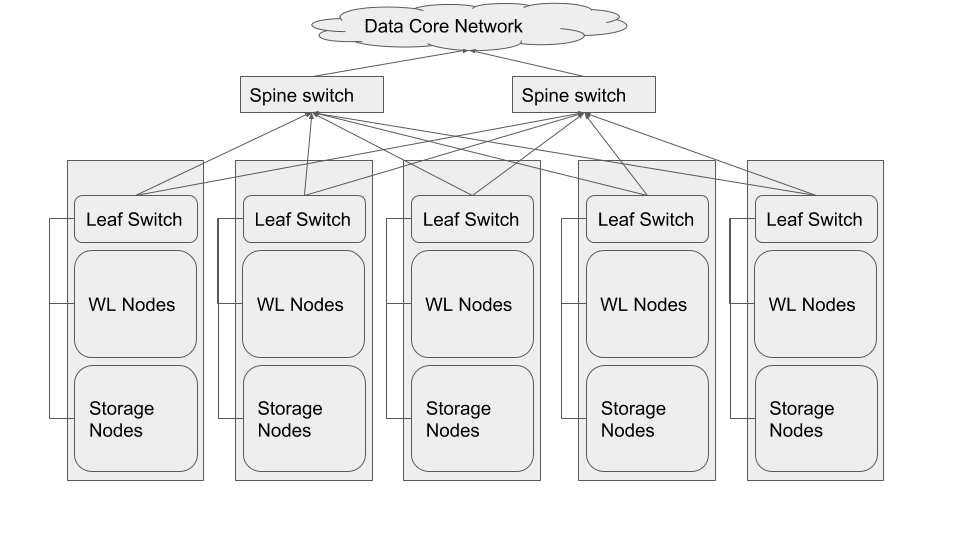
Physical Network Topology
The best network topology for Hadoop clusters is spine-leaf. Each rack of hardware has its own leaf switch and each leaf is connected to every spine switch. Ideally we would not like to have any oversubscription between spine and leaf. That would result in having full line rate between any two nodes in the cluster.
The choice of switches, bandwidth and so on would of course be predicated on the calculations in the previous section.
If the Storage nodes and the Workload nodes happen to reside in clearly separate racks, then it is necessary to ensure that between the workload rack switches and the Storage rack switches, there is at least as much uplink bandwidth as the theoretical max offered by the Storage cluster. In other words, the sum of the bandwidth of all workload-only racks needs to be equivalent to the sum of the bandwidth of all storage-only racks.
For instance, taking the example from the previous section, we should have at least 60 Gbps uplink between the Storage cluster and the workload cluster nodes.
If we are to build the desired network topology based on the sizing exercise from above, we would need the following.
| Layer | Network Per-port Bandwidth | Number of Ports required | Notes |
| Workload | 25 | 52 | Per sizing, we needed 20 Gbps per node. However, to simplify the design, let us pick single 25 Gbps ports instead of bonded pair of 10Gbps per node. |
| Storage | 25 | 43 | |
| Total Ports | 95 |
Assuming all the nodes are 2 RU in form factor, we would require 5 x 42 RU racks to house this entire set up.
If we place the nodes from each layer as evenly distributed across the 5 Racks as we can, we would end up with following configuration.
| Rack1 | Rack2 | Rack3 | Rack4 | Rack5 |
| Spine ( 20 x 100 Gbps uplink + 2 x 100 Gbps to Core) | Spine (20 x 100 Gbps uplink + 2 x 100 Gbps to Core) | |||
| ToR (18 x 25Gbps + 8 x 100 Gbps uplink) | ToR (20 x 25 Gbps + 8 x 100 Gbps uplink) | ToR (20 x 25 Gbps + 8 x 100 Gbps uplink ) | ToR (18 x 25 Gbps + 8 x 100 Gbps uplink) | ToR (20 x 25 Gbps + 8 x 100 Gbps uplink) |
| 10 x WL | 11 x WL | 11 x WL | 10 x WL | 11 x WL |
| 8 x Storage | 9 x Storage | 9 x Storage | 8 x Storage | 9 x Storage |
So that implies that we would have to choose ToR (Top of Rack) switches that have at least 20 x 25 Gbps ports and 8 x 100 Gbps uplink ports. Also the Spine switches would need at least 22 x 100 Gbps ports.
Using eight 100 Gbps uplinks from the leaf switches would result in almost 1:1 (1.125:1) oversubscription ratio between leaves (upto 20 x 25 Gbps ports) and the spine ( 4 x 100 Gbps per spine switch).
Mixing the Workload and Storage nodes in the way shown below, will help localize some traffic to each leaf and thereby reduce the pressure of N-S traffic (between Workload and
Storage clusters) patterns.
The following diagram illustrates the logical topology at a virtual machine level.
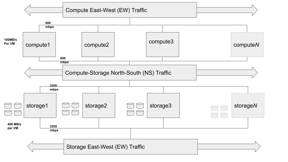
The Storage E-W, Compute N-S and Compute E-W components shown above are not separate networks, but are the same network with different traffic patterns, which have been broken out in order clearly denote the different traffic patterns.
