
Hash and range partitioning
The previous examples showed how the metrics table could be range partitioned on the time column, or hash partitioned on the host and metric columns. These
strategies have associated strength and weaknesses:
| Strategy | Writes | Reads | Tablet Growth |
|---|---|---|---|
|
|
✗ - all writes go to latest partition |
✓ - time-bounded scans can be pruned |
✓ - new tablets can be added for future time periods |
|
|
✓ - writes are spread evenly among tablets |
✓ - scans on specific hosts and metrics can be pruned |
✗ - tablets could grow too large |
Hash partitioning is good at maximizing write throughput, while range partitioning avoids issues of unbounded tablet growth. Both strategies can take advantage of partition pruning to optimize scans in different scenarios. Using multilevel partitioning, it is possible to combine the two strategies in order to gain the benefits of both, while minimizing the drawbacks of each.
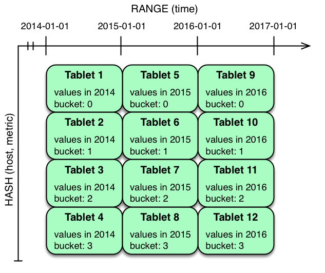
In the example above, range partitioning on the time column is combined with hash partitioning on the
host and metric columns. This strategy can be thought of as
having two dimensions of partitioning: one for the hash level and one for the range level. Writes
into this table at the current time will be parallelized up to the number of hash buckets, in
this case 4. Reads can take advantage of time bound and specific host and metric predicates to prune partitions. New
range partitions can be added, which results in creating 4 additional tablets (as if a new column
were added to the diagram).
